Dynamic Pricing Strategy in Python

Dynamic pricing is an application of data science that involves adjusting prices of products or services based on various factors in real time. It is used by businesses to optimize revenue and profitability by setting flexible prices that respond to market demand, customer behavior, and competitor pricing.

To implement a dynamic pricing strategy, businesses typically require data that can provide insights into customer behavior, market trends, and other influencing factors.

Dynamic Pricing Overview

The following are some of the factors that can be considered when implementing a dynamic pricing strategy:

• Historical sales data: This data can be used to understand how prices have affected demand in the past.

• Customer purchase patterns: This data can be used to understand how different customers respond to different prices.

• Market demand forecasts: This data can be used to predict future demand for products or services.

• Cost data: This data can be used to determine the minimum price that a business can charge for a product or service.

• Customer segmentation data: This data can be used to group customers into different segments based on their demographics, purchase behavior, and other factors.

• Real-time market data: This data can be used to track changes in demand, competitor pricing, and other factors that can affect prices.

Once a dynamic pricing strategy has been implemented, businesses can use it to adjust prices in real time to maximize revenue and profitability.

Here are some examples of how dynamic pricing can be used:

• A ride-sharing company can use dynamic pricing to increase prices during times of high demand, such as during rush hours or major events.

• A hotel can use dynamic pricing to increase prices during peak travel seasons.

• An e-commerce store can use dynamic pricing to offer discounts to customers who are more likely to abandon their carts.

Dynamic pricing can be a powerful tool for businesses that want to optimize their revenue and profitability. However, it is important to note that dynamic pricing can also lead to customer dissatisfaction if prices are perceived as being unfair or excessive. It is therefore important to carefully consider the factors that will affect customer perceptions of price fairness when implementing a dynamic pricing strategy.

This data can be used to train machine learning models that can predict optimal prices for products or services.

Lets start by importing the libraries we need!::

import pandas as pd
import plotly.express as px
import plotly.graph_objects as go

data = pd.read_csv("dynamic_pricing_Strategy_Dataset.csv")
print(data.head())

Output():

Number_of_Riders ... Historical_Cost_of_Ride

0 90 ... 284.257273

1 58 ... 173.874753

2 42 ... 329.795469

3 89 ... 470.201232

4 78 ... 579.681422

[5 rows x 10 columns]

Exploratory Data Analysis (EDA)

Gathering the descriptive statistics of the dataset::

print(data.describe())

Output():

Number_of_Riders ... Historical_Cost_of_Ride

count 1000.000000 ... 1000.000000

mean 60.372000 ... 372.502623

std 23.701506 ... 187.158756

min 20.000000 ... 25.993449

25% 40.000000 ... 221.365202

50% 60.000000 ... 362.019426

75% 81.000000 ... 510.497504

max 100.000000 ... 836.116419

[8 rows x 6 columns]

Investigating the relationship between expected ride duration and the historical cost of the ride::

fig = px.scatter(data, x='Expected_Ride_Duration', 
                 y='Historical_Cost_of_Ride',
                 title='Expected Ride Duration vs. Historical Cost of Ride', 
                 trendline='ols')
fig.show()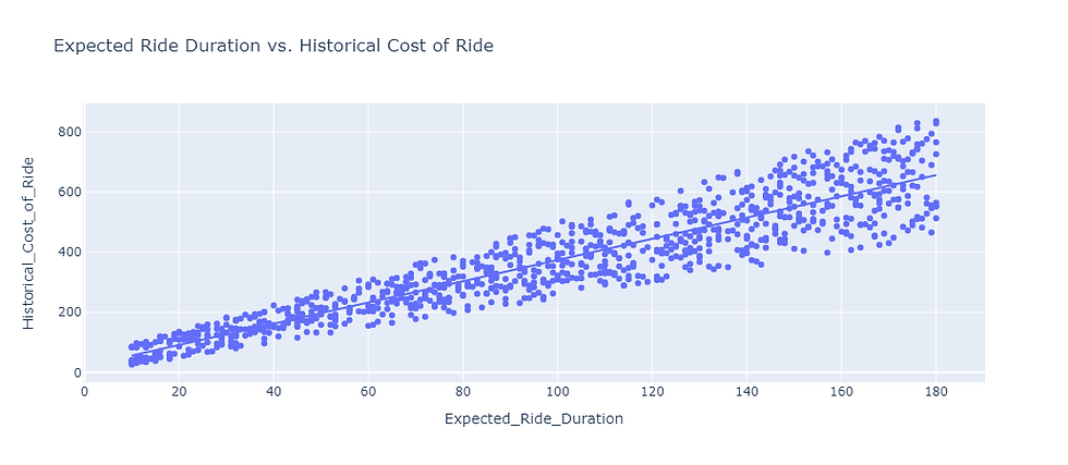

fig = px.box(data, x='Vehicle_Type', 
             y='Historical_Cost_of_Ride',
             title='Historical Cost of Ride Distribution by Vehicle Type')
fig.show()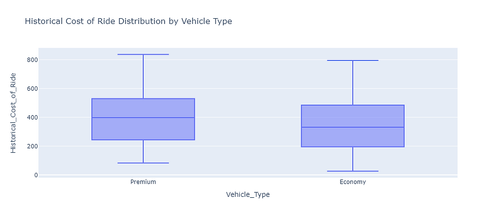

Performing a correlation matrix on the data::

corr_matrix = data.corr()

fig = go.Figure(data=go.Heatmap(z=corr_matrix.values, 
                                x=corr_matrix.columns, 
                                y=corr_matrix.columns,
                                colorscale='Viridis'))
fig.update_layout(title='Correlation Matrix')
fig.show()

Implementing a Dynamic Pricing Strategy

The company's current pricing model only considers the expected ride duration when setting prices. This means that the price of a ride is the same regardless of when or where the ride is taken. However, the data shows that demand and supply for rides can vary significantly depending on time of day, day of week, location, and other factors.

To address this, we will implement a dynamic pricing strategy that adjusts ride prices in real time based on demand and supply levels. This means that prices will be higher during times of high demand and lower during times of low demand. This will help to ensure that prices are fair and that riders are always able to find a ride, even during peak times.

Here are some examples of how dynamic pricing can work:

• During rush hour, when demand for rides is high, prices will be higher. This will incentivize more drivers to go online and provide rides, which will help to meet demand and ensure that riders can get to their destinations on time.

• On weekends, when demand for rides is lower, prices will be lower. This will make rides more affordable for riders and encourage them to use the service.

• In areas with a lot of competition, prices will be lower. This is because businesses will need to offer lower prices in order to compete with each other.

• 
  

Dynamic pricing is a powerful tool that can help businesses to optimize their revenue and profitability. By adjusting prices in real time based on demand and supply levels, businesses can ensure that they are always charging the right price for their products or services.

Now for the fun part!!!

Let's implement our dynamic pricing strategy using Python:

import numpy as np

# Calculate demand_multiplier based on percentile for high and low demand
high_demand_percentile = 75
low_demand_percentile = 25

data['demand_multiplier'] = np.where(data['Number_of_Riders'] > np.percentile(data['Number_of_Riders'], high_demand_percentile),
                                     data['Number_of_Riders'] / np.percentile(data['Number_of_Riders'], high_demand_percentile),
                                     data['Number_of_Riders'] / np.percentile(data['Number_of_Riders'], low_demand_percentile))

# Calculate supply_multiplier based on percentile for high and low supply
high_supply_percentile = 75
low_supply_percentile = 25

data['supply_multiplier'] = np.where(data['Number_of_Drivers'] > np.percentile(data['Number_of_Drivers'], low_supply_percentile),
                                     np.percentile(data['Number_of_Drivers'], high_supply_percentile) / data['Number_of_Drivers'],
                                     np.percentile(data['Number_of_Drivers'], low_supply_percentile) / data['Number_of_Drivers'])

# Define price adjustment factors for high and low demand/supply
demand_threshold_high = 1.2  # Higher demand threshold
demand_threshold_low = 0.8  # Lower demand threshold
supply_threshold_high = 0.8  # Higher supply threshold
supply_threshold_low = 1.2  # Lower supply threshold

# Calculate adjusted_ride_cost for dynamic pricing
data['adjusted_ride_cost'] = data['Historical_Cost_of_Ride'] * (
    np.maximum(data['demand_multiplier'], demand_threshold_low) *
    np.maximum(data['supply_multiplier'], supply_threshold_high)
)

As we can see, the code first calculates a demand multiplier by comparing the number of riders to percentiles representing high and low demand levels. If the number of riders is higher than the percentile for high demand, the demand multiplier is set to the number of riders divided by the high-demand percentile. Otherwise, if the number of riders is lower than the percentile for low demand, the demand multiplier is set to the number of riders divided by the low-demand percentile.

The code then calculates a supply multiplier by comparing the number of drivers to percentiles representing high and low supply levels. If the number of drivers is higher than the percentile for low supply, the supply multiplier is set to the high-supply percentile divided by the number of drivers. Otherwise, if the number of drivers is lower than the percentile for low supply, the supply multiplier is set to the low-supply percentile divided by the number of drivers.

Finally, the code calculates the adjusted ride cost for dynamic pricing. This is done by multiplying the historical cost of the ride by the maximum of the demand multiplier and a lower threshold (demand_threshold_low), and also by the maximum of the supply multiplier and an upper threshold (supply_threshold_high). This multiplication ensures that the adjusted ride cost captures the combined effect of demand and supply multipliers, with the thresholds serving as caps or floors to control the price adjustments.

Here is an example:

• If the number of riders is 100 and the percentile for high demand is 80, then the demand multiplier is set to 100/80 = 1.25.

• If the number of drivers is 50 and the percentile for low supply is 40, then the supply multiplier is set to 40/50 = 0.8.

• The adjusted ride cost would then be calculated by multiplying the historical cost of the ride by 1.25 and 0.8, which would give a final price of 1.0.

The thresholds (demand_threshold_low and supply_threshold_high) can be used to control the price adjustments. For example, if you want to cap the price increase to 20%, you would set demand_threshold_low to 1.2. This would ensure that the demand multiplier is never greater than 1.2, which would limit the price increase to 20%.

The thresholds can also be used to floor the price. For example, if you want to ensure that the price never falls below $10, you would set supply_threshold_high to 10. This would ensure that the supply multiplier is never less than 10, which would prevent the price from falling below $10.

After implement this dynamic pricing strategy we can now calculate the profit percentage we got::

# Calculate the profit percentage for each ride
data['profit_percentage'] = ((data['adjusted_ride_cost'] - data['Historical_Cost_of_Ride']) / data['Historical_Cost_of_Ride']) * 100
# Identify profitable rides where profit percentage is positive
profitable_rides = data[data['profit_percentage'] > 0]

# Identify loss rides where profit percentage is negative
loss_rides = data[data['profit_percentage'] < 0]


import plotly.graph_objects as go

# Calculate the count of profitable and loss rides
profitable_count = len(profitable_rides)
loss_count = len(loss_rides)

# Create a donut chart to show the distribution of profitable and loss rides
labels = ['Profitable Rides', 'Loss Rides']
values = [profitable_count, loss_count]

fig = go.Figure(data=[go.Pie(labels=labels, values=values, hole=0.4)])
fig.update_layout(title='Profitability of Rides (Dynamic Pricing vs. Historical Pricing)')
fig.show()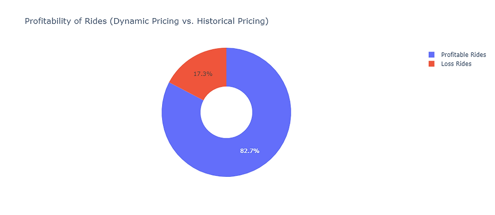

We can now take a look at the relationship between what the expected ride duration is and the cost of the ride based on the dynamic pricing strategy we employed::

fig = px.scatter(data, 
                 x='Expected_Ride_Duration', 
                 y='adjusted_ride_cost',
                 title='Expected Ride Duration vs. Cost of Ride', 
                 trendline='ols')
fig.show()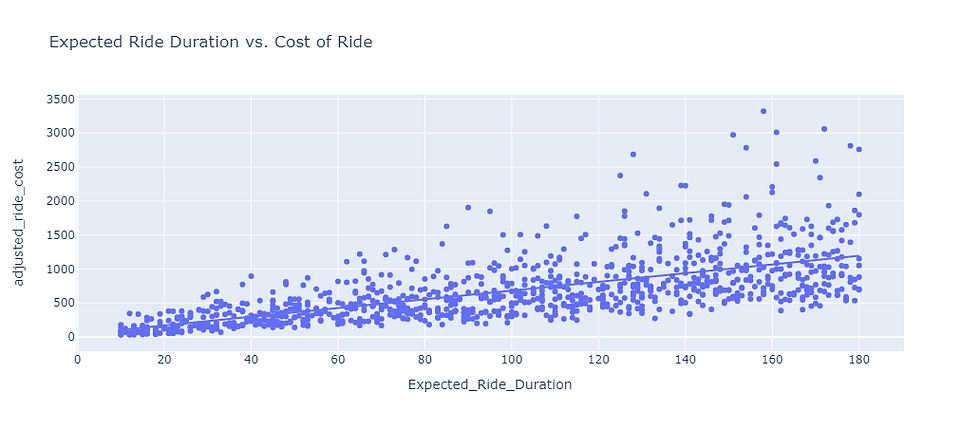

Training the Predictive Model

Before we train our Machine Learning Model, we must implement a data preprocessing pipeline to preprocess the data. This is debatebley one of the most important steps and something that should never be taken lightly regardless of how little you enjoy it.

import pandas as pd
import numpy as np
from sklearn.preprocessing import StandardScaler

def data_preprocessing_pipeline(data):
    #Identify numeric and categorical features
    numeric_features = data.select_dtypes(include=['float', 'int']).columns
    categorical_features = data.select_dtypes(include=['object']).columns

    #Handle missing values in numeric features
    data[numeric_features] = data[numeric_features].fillna(data[numeric_features].mean())

    #Detect and handle outliers in numeric features using IQR
    for feature in numeric_features:
        Q1 = data[feature].quantile(0.25)
        Q3 = data[feature].quantile(0.75)
        IQR = Q3 - Q1
        lower_bound = Q1 - (1.5 * IQR)
        upper_bound = Q3 + (1.5 * IQR)
        data[feature] = np.where((data[feature] < lower_bound) | (data[feature] > upper_bound),
                                 data[feature].mean(), data[feature])

    #Handle missing values in categorical features
    data[categorical_features] = data[categorical_features].fillna(data[categorical_features].mode().iloc[0])

    return data

Before moving forward, let's make this process easier for ourselves by converting vehicle type into a numerical feature considering that it is a valuable factor within our dataset and important to explore/investigate for better understanding of the story being told by the numbers::

data["Vehicle_Type"] = data["Vehicle_Type"].map({"Premium": 1, 
                                           "Economy": 0})

Now its time to split the data and train our Machine Learning model to predict the cost of a ride:

#splitting data
from sklearn.model_selection import train_test_split
x = np.array(data[["Number_of_Riders", "Number_of_Drivers", "Vehicle_Type", "Expected_Ride_Duration"]])
y = np.array(data[["adjusted_ride_cost"]])

x_train, x_test, y_train, y_test = train_test_split(x,
                                                    y,
                                                    test_size=0.2,
                                                    random_state=42)

# Reshape y to 1D array
y_train = y_train.ravel()
y_test = y_test.ravel()

# Training a random forest regression model
from sklearn.ensemble import RandomForestRegressor
model = RandomForestRegressor()
model.fit(x_train, y_train)

Now we have to test this Machine Learning model by giving it some input values::

def get_vehicle_type_numeric(vehicle_type):
    vehicle_type_mapping = {
        "Premium": 1,
        "Economy": 0
    }
    vehicle_type_numeric = vehicle_type_mapping.get(vehicle_type)
    return vehicle_type_numeric
  
# Predicting using user input values
def predict_price(number_of_riders, number_of_drivers, vehicle_type, Expected_Ride_Duration):
    vehicle_type_numeric = get_vehicle_type_numeric(vehicle_type)
    if vehicle_type_numeric is None:
        raise ValueError("Invalid vehicle type")
    
    input_data = np.array([[number_of_riders, number_of_drivers, vehicle_type_numeric, Expected_Ride_Duration]])
    predicted_price = model.predict(input_data)
    return predicted_price

# Example prediction using user input values
user_number_of_riders = 50
user_number_of_drivers = 25
user_vehicle_type = "Economy"
Expected_Ride_Duration = 30
predicted_price = predict_price(user_number_of_riders, user_number_of_drivers, user_vehicle_type, Expected_Ride_Duration)
print("Predicted price:", predicted_price)

Output():

Predicted price: [256.69895836]

This is a comparison of the actual predicted results::

import plotly.graph_objects as go

# Predict on the test set
y_pred = model.predict(x_test)

# Create a scatter plot with actual vs predicted values
fig = go.Figure()

fig.add_trace(go.Scatter(
    x=y_test.flatten(),
    y=y_pred,
    mode='markers',
    name='Actual vs Predicted'
))

# Add a line representing the ideal case
fig.add_trace(go.Scatter(
    x=[min(y_test.flatten()), max(y_test.flatten())],
    y=[min(y_test.flatten()), max(y_test.flatten())],
    mode='lines',
    name='Ideal',
    line=dict(color='red', dash='dash')
))

fig.update_layout(
    title='Actual vs Predicted Values',
    xaxis_title='Actual Values',
    yaxis_title='Predicted Values',
    showlegend=True
)

fig.show()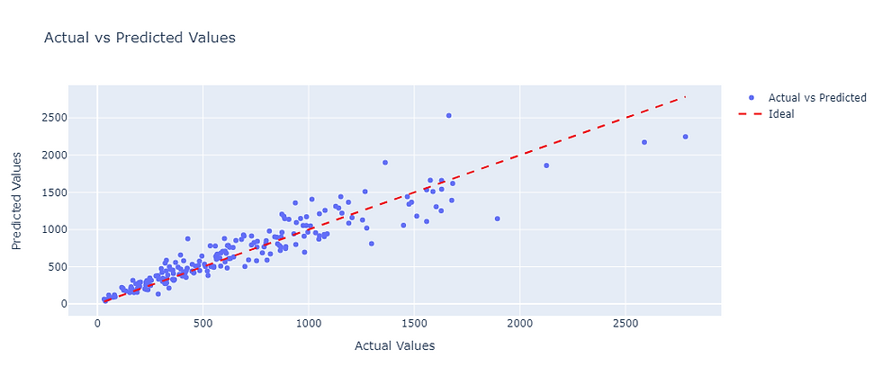

This is a methoud and use case of how Machine Learning can be used to implement a data-driven dynamic pricing strategy in Python.

Summary

The aim of a dynamic pricing strategy is to maximize revenue and profitability by pricing items at an optimum equilibrium balance the meets supply and demand dynamics. This allows for businesses to adjust prices dynamically based on factors such as the time of day, day of the week, customer segments, inventory levels, seasonal functions, competitor pricing, and market conditions. As we can see this is a useful tool in understanding and uncovering how ones data can be used to drive optimal results and lead to ideal profit margins, especially in times of uncertainty where every decision can have a make or break outcome on a companys'/brands' success!